Big O Notation - Analyzing Time Complexity in Elixir
Big O notation, a fundamental concept in computer science and mathematics, is widely used to analyze the performance and efficiency of data structures and algorithms, providing a way to express the growth of their runtime or space complexity as a function of input size.
Big O notation, a fundamental concept in computer science and mathematics, is widely used to analyze the performance and efficiency of data structures and algorithms, providing a way to express the growth of their runtime or space complexity as a function of input size.
Big O Notation is a broad topic that can be difficult to navigate so we'll narrow the lens to focus on some basic rules for analyzing Time Complexity with Elixir, and introduce some general categories using examples and explanations.
Time Complexity
In the context of Big O notation, time complexity refers to the measure of the amount of "time" an algorithm takes to execute as a function of the size of its input.
It essentially answers the question: How will an algorithm's performance change as the data increases?
Basic Guidelines
There are some key points or rules to remember when it comes to analyzing and describing time complexity:
- Time Complexity describes how the number of steps or operations change as input size changes, not the "pure time" an algorithm takes to complete. The same code can run differently depending on the hardware.
- Time Complexity generally refers to the worst-case scenario. Knowing how inefficient an algorithm can become can strongly impact choices by preparing for the worst.
- Big O Notation ignores constants and describes algorithms in general categories. Algorithms can perform drastically differently as data changes, so describing subtle differences within categories becomes unnecessary.
Let's consider these guidelines as we look at a few of the most common algorithm categories.
Constant Time Complexity - O(1)
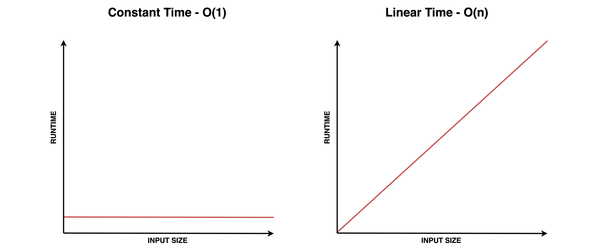
Constant time operations are represented in Big O notation as: O(1). This means that the number of steps required to perform the operation remains constant regardless of the input size. This is the most efficient algorithm category.
In Elixir, accessing an element in a Tuple has constant time complexity. In other words, random access can be performed in the same number of steps regardless of data size.
Example 1
Here's a basic, contrived example to start reviewing Elixir code:
defmodule BigOnion do
  def constant_time(input_tuple, index) do
    elem(input_tuple, index)
  end
end

input_tuple = {"a", "b", "c"}
BigOnion.constant_time(input_tuple, 1)Looking at this code, let's ask the question: How will performance change as the data increases?
- We know the length of the tuple is three so
n = 3(nis generally used to describe the input data size) - We know that we can access any element in the tuple in a single step
| n Elements | # Steps |
|---|---|
| 1 | 1 |
| 10 | 1 |
| 100 | 1 |
| 1000 | 1 |
Because the possible number of steps needed remains constant as data increases, this algorithm can be described as O(1) or as having Constant Time Complexity.
Example 2
Using the same example above, what if we needed uppercase values?
defmodule BigOnion do
  def constant_time(input_tuple, index) do
    input_tuple
    |> elem(index)
    |> String.upcase()
  end
end

input_tuple = {"a", "b", "c"}
BigOnion.constant_time(input_tuple, 1)Again, let's ask the question: How will performance change as the data increases?
- the length of the tuple is three so
n = 3 - we can access any element in the tuple in a single step
- upcasing the string is another step
| n Elements | # Steps |
|---|---|
| 1 | 2 |
| 10 | 2 |
| 100 | 2 |
| 1000 | 2 |
This time, the algorithm is O(2) which still falls into the Constant Time category.
O(1).Let's look at another example that will help illustrate why these guidelines are useful when analyzing complexity.
Linear Time Complexity - O(n)
Linear time complexity means that the number of operations increases linearly with the input size – as the input data increases, the number of operations needed will increase at the same rate.
Example 1
Here's the same basic algorithm, this time using a List (singly linked list) as the underlying data structure where lookups have Linear Time Complexity:
defmodule BigOnion do
  def linear_time(input_list, target) do
    Enum.at(input_list, target)
  end
end

input_list = ["a", "b", "c"]
BigOnion.linear_time(input_list, 1)Again, let's ask the question: How will performance change as the data increases?
- We know the input List length is 3, so
n = 3 - To access a random element on a List data-structure, the VM must start at index
0and traverse through the list until it reaches the given index. - The number of possible steps will increase as the length of the list increases.
| n Elements | # Possible Steps |
|---|---|
| 1 | 1 |
| 10 | 10 |
| 100 | 100 |
| 1000 | 1000 |
Worst-Case Scenario
In the best case, the value at index 0 or head of the list is requested, which will take a single step O(1). In the worst-case, the value at the end of the list will be requested and take 3 steps O(3).
When the length or size of data increases, the worst-case scenario increases to the new length of the List – so rather than using a dynamic value to describe the possible number of steps, Linear Time Complexity is represented as O(n) where n is the size of the input data.
Example 2
Let's add another step to upcase all the values before selecting the target:
defmodule BigOnion do
  def linear_time(input_list, target) do
    input_list
    |> Enum.map(fn x -> String.upcase(x) end)
    |> Enum.at(target)
  end
end

input_list = ["a", "b", "c"]
BigOnion.linear_time(input_list, 1)
In this (obviously flawed) approach, n = 3 and now, there are two operations that will traverse the entire list, so we'll have 2 * 3 steps or O(2n).
How will this algorithm's performance change as the data increases?
As the input data increases, only n will change. Two full traversals are constant – so just like the previous example, this algorithm starts as O(2n) and after dropping constants falls into the Linear Time Complexity general category: O(n).
Comparing Algorithms
We're starting to see why it's unnecessary to describe an algorithm with details such as constants when comparing two examples with different runtime complexity:
- Tuple-based - Constant Time
O(2)worst-case scenario. - List-based - Linear Time
O(2n)worst-case scenario.
Even with multiple steps and as data increases, an algorithm with Constant Time Complexity will be more efficient than one with Linear Time Complexity and therefore O(1) is sufficient to describe the first algorithm compared to O(n).
After analyzing and comparing these two examples, we have enough information to choose an implementation and can communicate the performance characteristics of each approach.
Logarithmic Time Complexity - O(log n)
Logarithmic time complexity means that the number of operations increases logarithmically with the input size – this may not be clear so let's start with defining logarithms and then analyze some examples.
Logarithms
A logarithm is a mathematical function that determines the exponent to which a base must be raised in order to produce a given number.
Exponents are used to represent the repeated multiplication of a number by itself. For example, 23 means 2 multiplied by itself 3 times, i.e., 2 * 2 * 2 = 8.
Logarithms are the inverse of exponents, allowing us to determine the exponent needed to raise a base number to obtain a specific value. For instance, here the base is two: log2(8) = 3, since 23 = 8. Another way of thinking about this is to ask the question:
How many times do we need to divide 8 by 2 until we end up with 1?
Let's look at an example to unpack this more.
Binary Search Example
Binary search is a classic example of logarithmic time complexity. This is a slightly more complex algorithm so keep the preceding guidelines and ideas in mind as we step through it.
O(log n) it's short for O(log2 n) where the base 2 is omitted for convenience.Here, we're searching a tuple data structure for a particular value, then returning the index where it was found:
defmodule BigOnion do
  def binary_search(data, target) do
    low = 0
    high = tuple_size(data) - 1
    do_binary_search(data, target, low, high)
  end

  defp do_binary_search(data, target, low, high) when low <= high do
    mid = div(low + high, 2)

    case elem(data, mid) do
      value when value == target ->
        mid

      value when value < target ->
        do_binary_search(data, target, mid + 1, high)

      value when value > target ->
        do_binary_search(data, target, low, mid - 1)
    end
  end

  defp do_binary_search(_, _, _, _), do: :not_found
end

sorted_data = {1, 2, 3, 4, 5, 6, 7, 8}
BigOnion.binary_search(sorted_data, 7)First, this algorithm expects values to be sorted. It will find the index at the midpoint by dividing the dataset in half – check the value, then either return the target's index or recursively call itself with the left or right subset of values.
Each call will eliminate approximately half of the possible values and thereby, half of the possible steps. So let's again ask the following question:
How will this algorithm's performance change as the data increases?
| n elements | possible steps |
|---|---|
| 8 | 3 |
| 16 | 4 |
| 32 | 5 |
Doubling the size of input data increases the number of possible steps by only one.
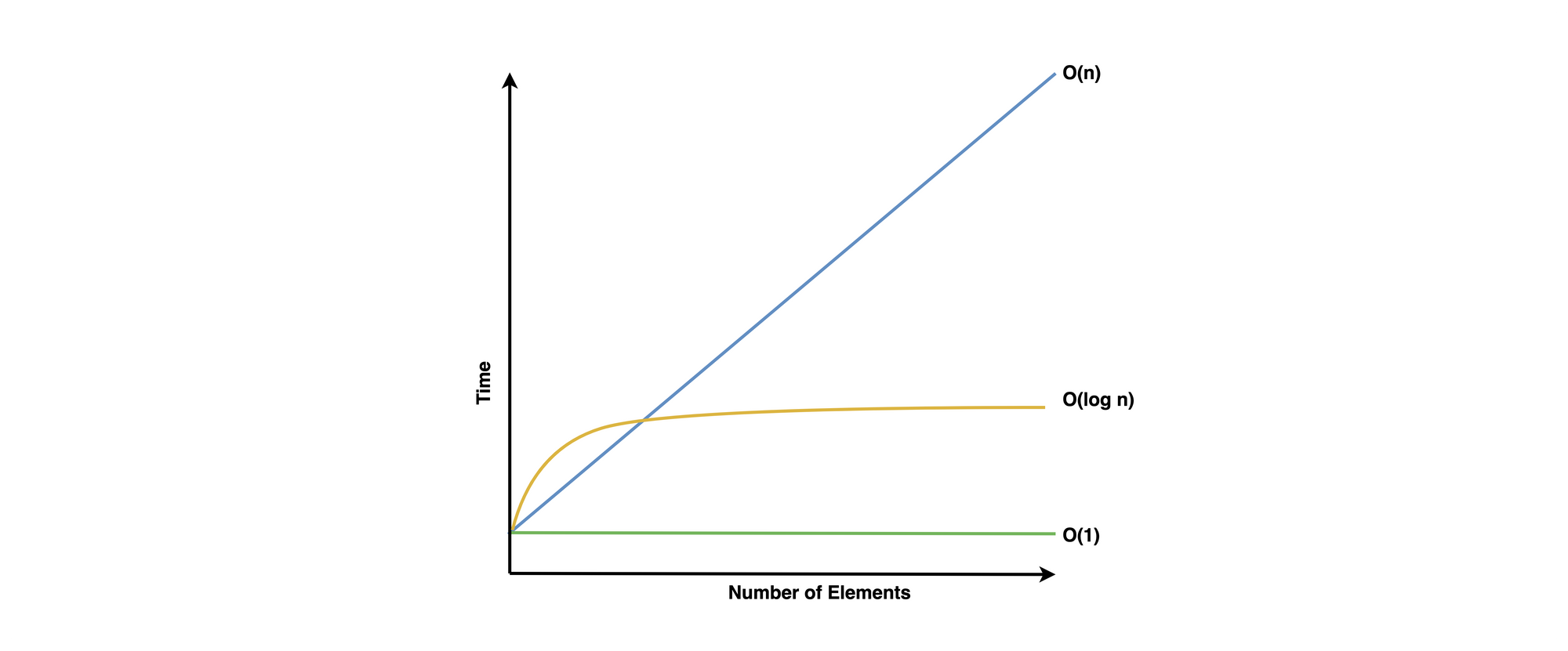
From this simple graph, we can see that Logarithmic Time Complexity falls roughly between Constant and Linear Time Complexity.
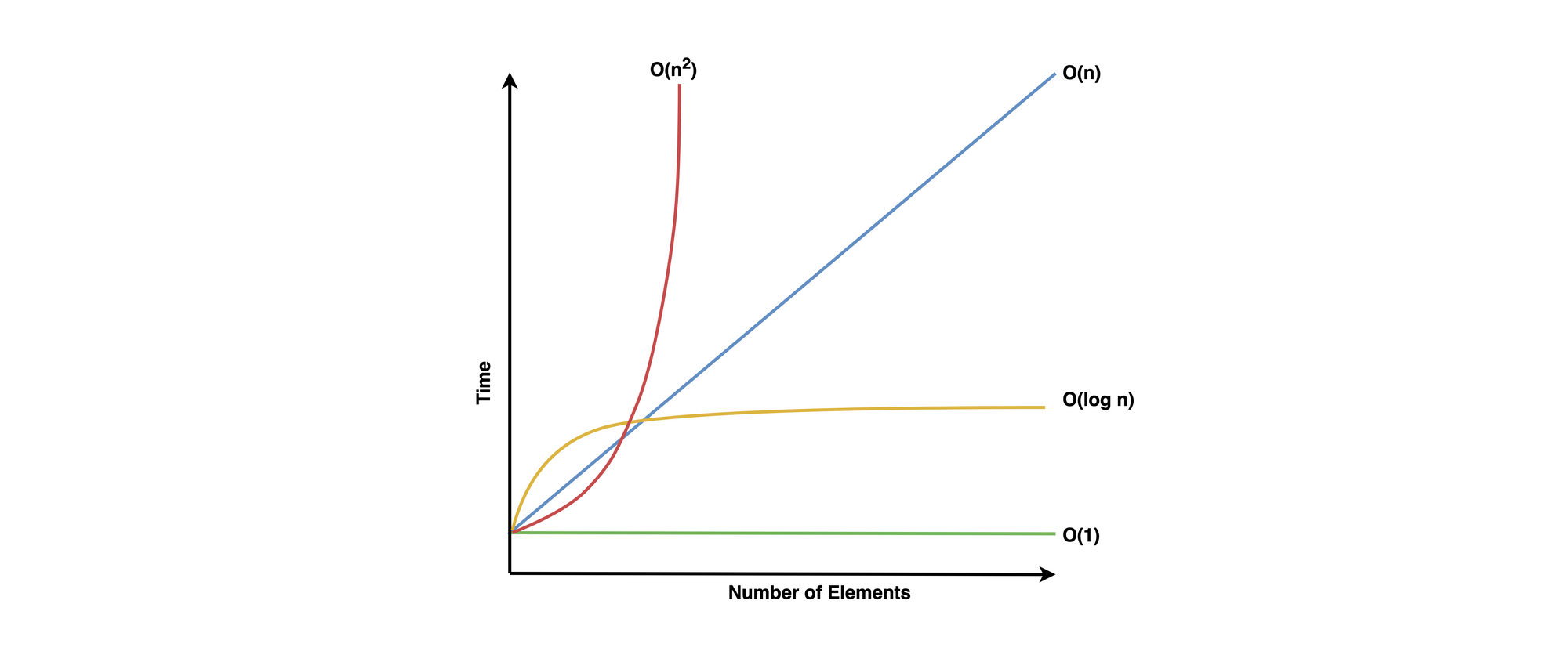
O(n) because in the worst-case scenario, the entire list would be traversed in search of the target.Quadratic Time Complexity - O(n2)
An algorithm with Quadratic Time Complexity means the number of steps it takes to accomplish a task is the square of n.
Duplicates Example
Let's look at an algorithm that checks if a list has duplicate values:
defmodule BigOnion do
  def has_duplicate_value?(data) do
    data
    |> Enum.with_index()
    |> Enum.flat_map(fn {val1, index1} ->
      data
      |> Enum.with_index()
      |> Enum.map(fn {val2, index2} ->
        if val1 == val2 and index1 != index2 do
          true
        else
          false
        end
      end)
    end)
    |> Enum.any?(&(&1 == true))
  end
end

data = [1,2,3,4,3]
BigOnion.has_duplicate_value?(data)This algorithm will traverse the full list, and for each element in the list, it will traverse the entire list again in nested traversals. This is normally a signal that the algorithm has Quadratic Time Complexity.
Analysis
Let's analyze this algorithm in a little more detail where n = 5:
Outer:
- adding indices to the list -
5 steps - mapping over the list -
5 steps - check for any truthy values -
5 steps - total:
3 * 5 steps
Nested:
- adding indices to the list -
5 steps - mapping over the list -
5 steps - comparison -
1 step - total:
2 * 5 + 1 steps
Total: 3n * 2n + 1
And as we've discussed previously, rather than describing this algorithm as 3n * 2n + 1, we can omit constants and say that it's O(n2).
Wrapping up
To recap – here are the guidelines we mentioned when analyzing time complexity for Big O notation:
- Time Complexity describes how the number of steps or operations change as input size changes, not the "pure time" an algorithm takes to complete. The same code can run differently depending on the hardware.
- Time Complexity generally refers to the worst-case scenario. Knowing how inefficient an algorithm can become can strongly impact choices by preparing for the worst.
- Big O Notation ignores constants and describes algorithms in general categories. Algorithms can perform drastically differently as data changes, so describing subtle differences within categories becomes unnecessary.
And here are the four general categories we covered:
- Constant Time -
O(1) - Logarithmic Time -
O(log n) - Linear Time -
O(n) - Quadratic Time -
O(n2)
Big O notation is a useful tool for designing algorithms, choosing data structures, and solving programming problems but just like any other skill, learning to analyze code and communicate effectively about performance can take some practice.
I hope you found this introductory guide helpful.
Book
I'm in the process of writing a book for Elixir/Erlang developers to dive deeper into functional data structures and algorithms.
Subscribe to the free newsletter for updates and progress!
-- Troy
Twitter: @tmartin8080 | ElixirForum